CSSS 508, Week 3
Rebecca Ferrell
April 13, 2016
Weaning you off of spreadsheets
Today we'll talk about dplyr: a package that does in R just about any calculation you've tried to do in Excel, but more transparently, reproducibly, and safely. Don't be the sad research assistant who made this mistake (Reinhart and Rogoff):

Modifying data frames with dplyr
Filtering rows (subsetting)
Recall last week we used the filter command to subset data like so:
library(dplyr)
library(gapminder)

Canada <- gapminder %>%
    filter(country == "Canada")
Excel analogue:

%in%
What values are out there? Use distinct
Time to talk about pipes (%>%)
Piping
Sampling rows: sample_n
Sorting: arrange
Keeping columns: select
Dropping columns: select
Helper functions for select
select() has a variety of helper functions like starts_with, ends_with, and contains, or giving a range of continguous columns startvar:endvar. These are very useful if you have a “wide” data frame with column names following a pattern or ordering. See ?select.

(US Dept. of Education “College Scorecard” data: > 100 columns)
Renaming columns with select
Safer: rename columns with...rename
Column naming practices
Column name with space example
Create new columns: mutate and transmute
Thing you do in spreadsheets: add column to data, drag down.

dplyr way: add new columns to a data frame using mutate. (Add new columns and drop old ones using transmute.)
mutate example
ifelse()
Summarizing with dplyr
General aggregation: summarize
summarize takes your rows of data and computes something across them: count how many rows there are, calculate the mean or total, etc. You can use any function that aggregates multiple values into a single one (like sd).
In a spreadsheet:
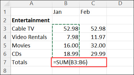
Summarize example
Avoiding repetition: summarize_each
Splitting data into groups: group_by
The special function group_by() changes how functions operate on the data, most importantly summarize. These functions are computed within each group as defined by variables given, rather than over all rows at once. Typically the variables you group by will be integers, factors, or characters, and not continuous real values.
Excel analogue: pivot tables
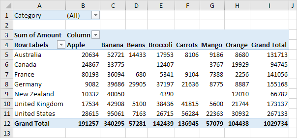
group_by() example
Window functions
Lab break!
Joining data frames
When do we need to join tables?
- Want to make columns using criteria too complicated for
ifelse() - Combine data stored in separate places: e.g. UW registrar information with student homework grades
Excel equivalents: VLOOKUP, MATCH

Joining: conceptually
Types of joins: rows and columns to keep
Matching criteria
nycflights13 data
Join example #1
Join example #2
Join example #3
Wind gusts and delays

Redo after removing extreme outliers, just trend
Wind gusts and delays: mean trend
